Google Summer of Code Final Work Product#
Organization: Python Software Foundation
Sub-Organization: DIPY
Project: AI/ML in diffusion MRI processing
Repository: TractoEncoder GSoC
Project Abstract#
The objective of the project is to generate synthetic human tractograms with tuneable age and neurodegeneration status properties, using deep learning models. The project is inspired by the FINTA and GESTA works, which propose a generative method using an AutoEncoder architecture for unconditional tractogram generation, and a robust sampling strategy, respectively. In our case, we replicated the results of the FINTA paper AutoEncoder in the FiberCup dataset using TensorFlow2 (TF2) as the deep learning backend, instead of the original PyTorch backend. We also investigated how to condition the AutoEncoder architecture on scalar and categorical variables to support conditional tractogram generation on age and neurodegeneration status. Finally, we also explored the use of Variational AutoEncoders, Regression AutoEncoders, and Adversarial AutoEncoders for tractogram generation under the mentioned conditions.
Proposed Objectives#
Replicate the results of the AutoEncoder architecture in the FINTA paper using TensorFlow2 as the deep learning backend.
Obtain publicly available data from the ADNI, the FiberCup and the ISMRM2015 tractography challenge to compute tractograms for training the deep learning models.
Integrate the replicated unconditional AutoEncoder architecture and sampling algorithm into DIPY to generate synthetic human tractograms, after training it with extensive human tractogram data.
Investigate how to condition the AutoEncoder architecture on scalar and categorical variables to support conditional tractogram generation on age and neurodegeneration status.
Implement a conditional AutoEncoder architecture that can generate synthetic tractograms conditioned on age and neurodegeneration status.
Modified Objectives (Additional)#
Investigate the use of Variational AutoEncoders (VAE) for unconditional tractogram generation based on the FINTA architecture.
Investigate the use of Conditional Variational AutoEncoders (CVAE) for conditional tractogram generation based on the FINTA architecture.
Investigate the possibility to condition the tractogram generation on the fiber bundle for additional control over the process and the data generation, using Adversarial AutoEncoders with attribute-based regularization.
Objectives Completed#
Literature Review on synthetic tractography generation using AutoEncoders. Main inspirations:
The FINTA and GESTA papers because they provide a relatively simple AE architecture with an open source sampling algorithm, easy to reuse.
Variational AutoEncoders for Regression, which provided a good starting point for conditional Variational AutoEncoders with direct application to brain aging, related to the project’s objectives.
Attribute-based Regularization of latent spaces for variational AutoEncoders and Adversarial AutoEncoders, which inspired the use of Attribute-based regularization for conditioning on a continuous variable (age); and the use of adversarial training for conditioning on categoric variables (fiber bundle or neurodegeneration status), respectively.
Replicated the FINTA architecture originally implemented in PyTorch (vanilla AutoEncoder, not variational) using TensorFlow2+Keras. Validated the results using the FiberCup dataset. The model is found in the
ae_model.pymodule of the TractoEncoder GSoC repository. The architecture can be summarized as in the following image:
Weight and bias initializers are different in PyTorch compared to TensorFlow2, so the PyTorch behavior was replicated using custom initializers. Different weight & bias initialization strategies can lead to drastically different training results, so this step took extra care.
The upsampling layers of the Decoder block use linear interpolation in PyTorch by default, whereas in TensorFlow2, there is no native implementation for this, and nearest neighbor (NN) interpolation is used instead. This is a significant difference in implementations, and to replicate the PyTorch behavior a custom linear interpolating upsampling layer was implemented in TF2. However, after training with both NN and linear interpolation, the results were very similar, so the custom layer was not used in the final implementation. This work was developed in a separate branch.
Training was run for 120 epochs, using a data set containing plausible and implausible streamlines. All the training experiments in my GSoC work were done with this data set. The figure below shows a summary of the replication results, which consist of running a set of unseen plausible streamlines through the model (encoder and decoder):

We see that the Keras result is very similar to the PyTorch result, though the fiber crossings are not as well resolved in the Keras result. This is not a thing to worry since this is not systematic, as seen in other sets of unseen data.#
Implemented a Variational AutoEncoder (VAE) architecture based on the FINTA AE architecture.
After thorough discussion with my mentors, we decided that regularizing the latent space could be a good idea due to two reasons: to avoid “white spaces” in the latent space it that could lead undefined points due to the possible discontinuity of the space; and to prevent the model from learning the identity function, what is a known issue with unregularized AutoEncoders, though it does not always happen. The only addition to the original AE architecture was the inclusion of the Kullback-Leibler divergence loss term in the loss function, and two dense layers after the convolutional layers of the encoder, to output the \(\mu\) and \(\sigma^2\) of the latent space vector \(z\).
The model is found in the
vae_model.pymodule of the TractoEncoder GSoC repository. The architecture can be summarized in the figure below:
It was necessary to implement Batch Normalization after the Encoder convolutional layers and exponential operator clipping, to prevent gradient explosion while training the model. The figure above displays that the encoder outputs the variance of the latent space vector (\(\sigma^2\)), though it is a common practice to output the log-variance instead. This leads to using \(\sigma = e^{\frac{1}{2}\text{log}{\sigma^2}}\), which can get numerically quite unstable as it can shoot up very quickly when a sufficiently big log-variance is input. This modification allowed stable training and it was a major contribution to the robustness of the architecture. Shout out to my lab colleague Jorge for the ideas and discussions on the topic.
Weighing the Kullback-Leibler loss component was also implemented, based on the Beta-VAE work, aiming for a stronger disentanglement of the latent space. However, this parameter was never explored (it was always set to 1.0) due to its trade-off with the reconstruction accuracy, but it is a potential improvement for future work in the context of hyperparameter optimization.
The figure below shows a summary of the VAE results, also using the FiberCup dataset:
The bottom row shows a set of unseen test data, and its reconstruction, after running it through the model (encode & decode). We can see that the reconstruction fidelity is not as good as the vanilla AE, but it is still acceptable, considering that the model was only trained for 120 epochs, which took around 2 hours in my GPU-less laptop.#
Implemented a conditional Variational Autoencoder (condVAE) architecture based on the Variational AutoEncoders for Regression paper.
The model is found in the
cond_vae_model.pymodule of the TractoEncoder GSoC repository. The model was trained on the FiberCup dataset, and the conditioning variable in this case was chosen to be the length of the streamlines, hypothesizing that this is a relatively simple feature to capture by the model based on their geometry. The majority of the architecture is based on the VAE from the previous point (also based on the FINTA architecture), to which I added two dense layers to output the \(\sigma_r\) and \(\text{log}\sigma^2_r\) of the regressed attribute, as well as the generator block. A diagram of the architecture can be seen below:
Implemented validation strategies of the condVAE model to check that the model can capture the variability of the conditioning variable.
By exploring the latent space of the VAE and condVAE models, we can compare the organization of the samples in the latent space, and see whether there is a difference aligned with the conditioning variable. After training for 64 epochs just to check how the model was progressing, I projected the 32-dimensional latent space using the t-SNE algorithm, to visualize it easily. This particular algorithm was chosen due to its popularity, speed, and availability in widespread libraries like scikit-learn. The projections only show the plausible fibers. The results are shown in the figures below:
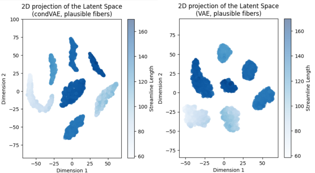
We observe that the condVAE model clusters are elongated, which made us arrive to the conclusion that the conditioning might be doing something, but it was yet not clear if it was what we wanted to achieve. Using the length of the streamlines as the conditioning variable was not the best choice because this parameter is very consistent inside each bundle of the FiberCup dataset, and knowing that each cluster corresponds to a bundle (7 clusters, 7 morphologically different bundles), we had not foreseen that each cluster was going to have a consistent coloring for the length attribute (which is quite obvious, once you know this). The conclusion of this exercise was that the model was doing something differently compared to the VAE, which could be good, or not.#
Another aspect to validate was the capability of the model to correctly capture the conditioning variable in the training data. To do so, we retrained the model until we got a close-to-zero label loss (in charge of capturing this variability), and computed the \(MSE\) and the \(R^2\) metrics between the predicted and the true conditioning variable. In addition, we plotted the latent space 2D projection again. The results are shown in the figure below:
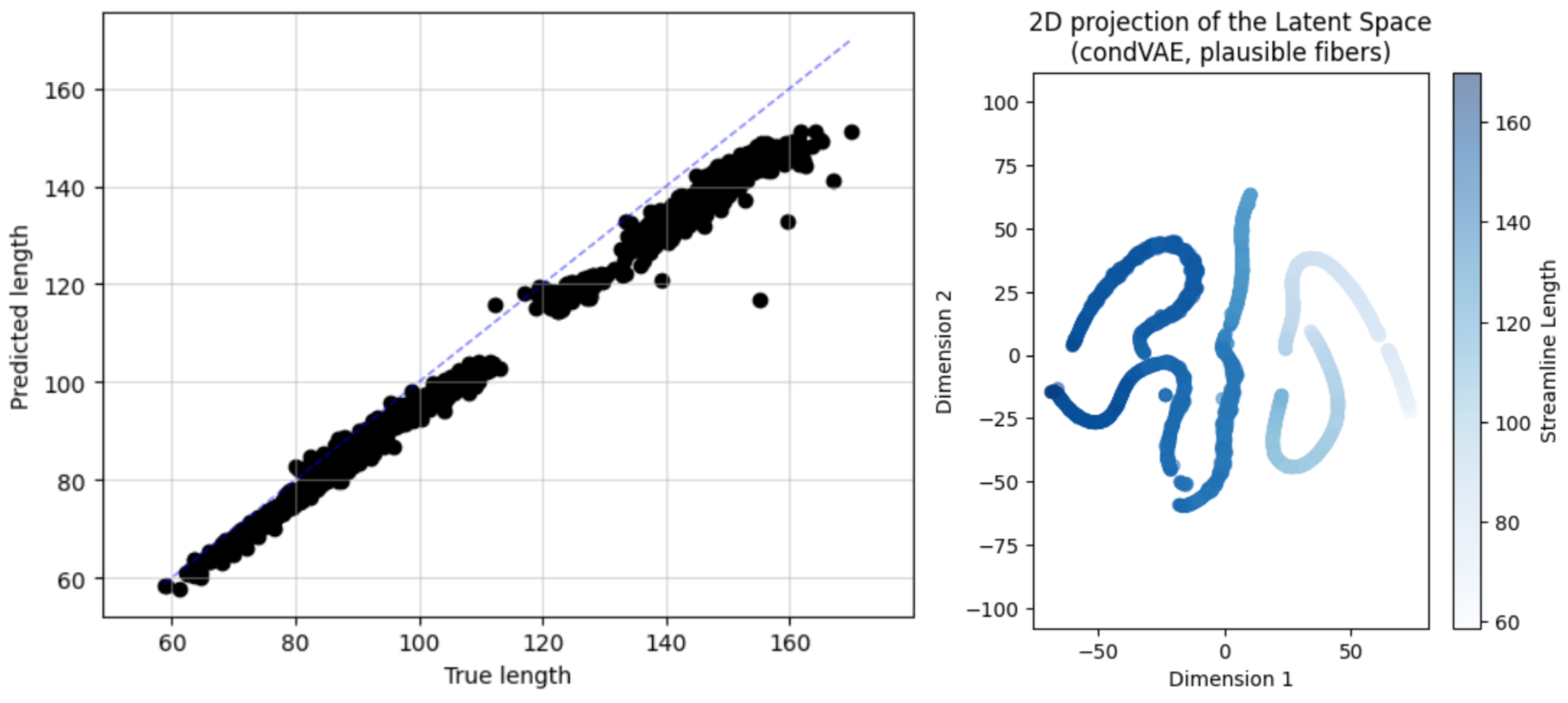
We got an \(\text{MSE}=50.371\) and an \(R^2=0.941\), and the latent space was organized in 7 clusters (the middle line is actually 2 lines, there is a small separation in the middle), which correspond to the 7 bundles of the FiberCup dataset, thus we saw that the model was indeed capable of predicting the conditioning variable fairly well. From left to right, the streamlines get shorter (the color gets lighter) with a gradient in the latent space that is aligned with the conditioning variable. The morphology of the leftmost clusters would indicate that they are the most variable in length, contrary to the middle clusters (the straighter lines), which are almost in the same horizontal coordinate. Having the t-SNE projection aligned with the conditioning variable is a good sign, that some dimension in the latent space was correctly tied to the conditioning variable.#
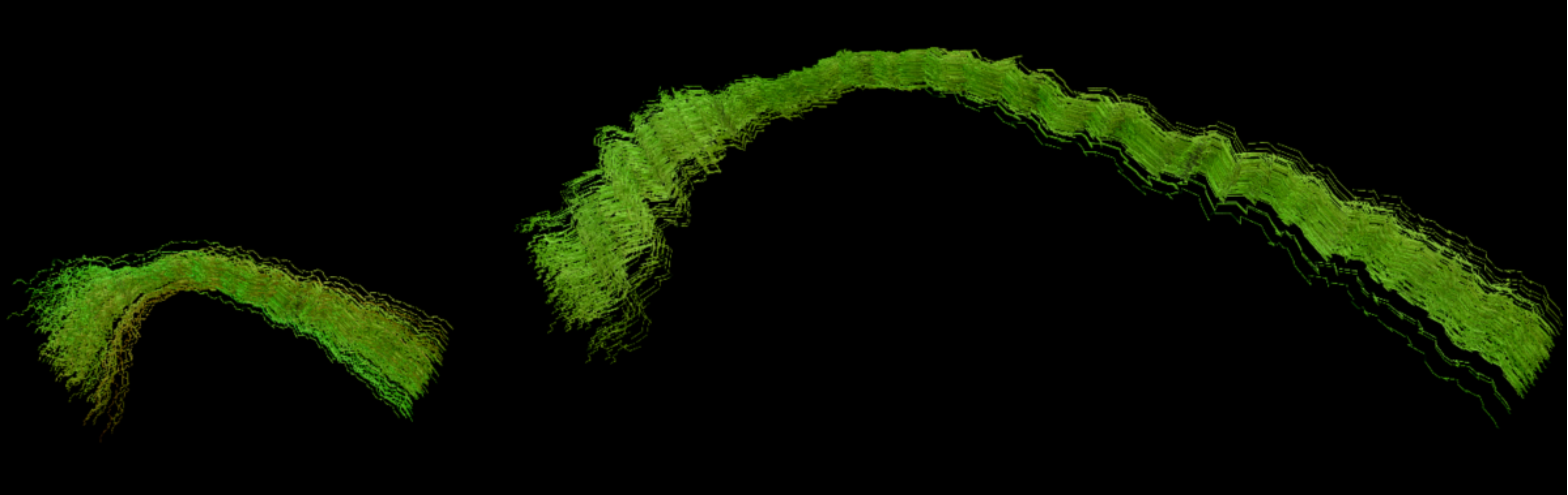
As the last experiment to validate the capabilities of this model and architecture, I proceeded to generate synthetic streamlines conditioned on their length. Theoretically, the model should be able to generate samples of specific lengths, and each length should be related to a specific bundle, as shorter fibers look different than the longer ones. Nonetheless, there was a major flaw in the generative process that my mentor Jong Sung had detected just before going into this step. When looking at the architecture of the model, the generative process would start from the \(r\) variable, setting it to a desired quantity, and then running the input through
D5andD6, then adding noise like \(z=\mu_{p_z}+\sigma_{p_z}\odot\epsilon\), and decoding this output.Since the generator block is trying to predict the whole latent vector \(z\) from a single number (\(r\)), the model was going to probably have trouble getting the necessary geometrical variability, and overall problems for generating different things from the same number. The model was not designed for generating samples and rather to regress their associated conditioning variable, and this was a major issue that had not been foreseen. This was a good lesson to learn, and it was a good opportunity to think about the importance of the generative process in the model design, and how it should be aligned with the model’s objectives. The figure below shows a set of generated samples of lengths 30 and 300 (left and right), seeing that the model was generating a very constant shape, only scaled in length:
Implemented an Adversarial AutoEncoder (AAE) architecture.
As the previous efforts with the conditional VAE were unfruitful, we resorted to using an adversarial framework. This was driven by the following reasons:
The adversarial nature of the architecture implicitly introduces a prior to the data, so regularization with variational methods is not necessary, so the architecture and the loss computation of the model is simpler.
It is easier to understand, because the original authors of the implemented conditional VAE did not provide a clear derivation of the loss function, so my understanding of its underlying mechanisms is not as deep as I would need to tune its behavior effectively. All in all, the adversarial framework is way more intuitive (at least for me).
It is widespread and there are many resources out there to understand it and implement it. What is more, I quickly found several implementations of adversarial AutoEncoders in TensorFlow with a basic search in Google. I need to read through them and filter which one is the best for me.
For sure there are ways to condition the network on categorical and continuous variables, which would be really convenient to condition both on the bundle and the attribute of the data. It had not been possible with the conditional VAE implementation, as it only conditions on the attribute. This would provide greater control when sampling from the latent space, and it would be more aligned with the original project proposal, which includes a continuous variable (age) and a categorical variable (neurodegeneration status).
The model is found in the
adv_ae_model.pymodule of the TractoEncoder GSoC repository. The proposed architecture can be summarized in the figure below:`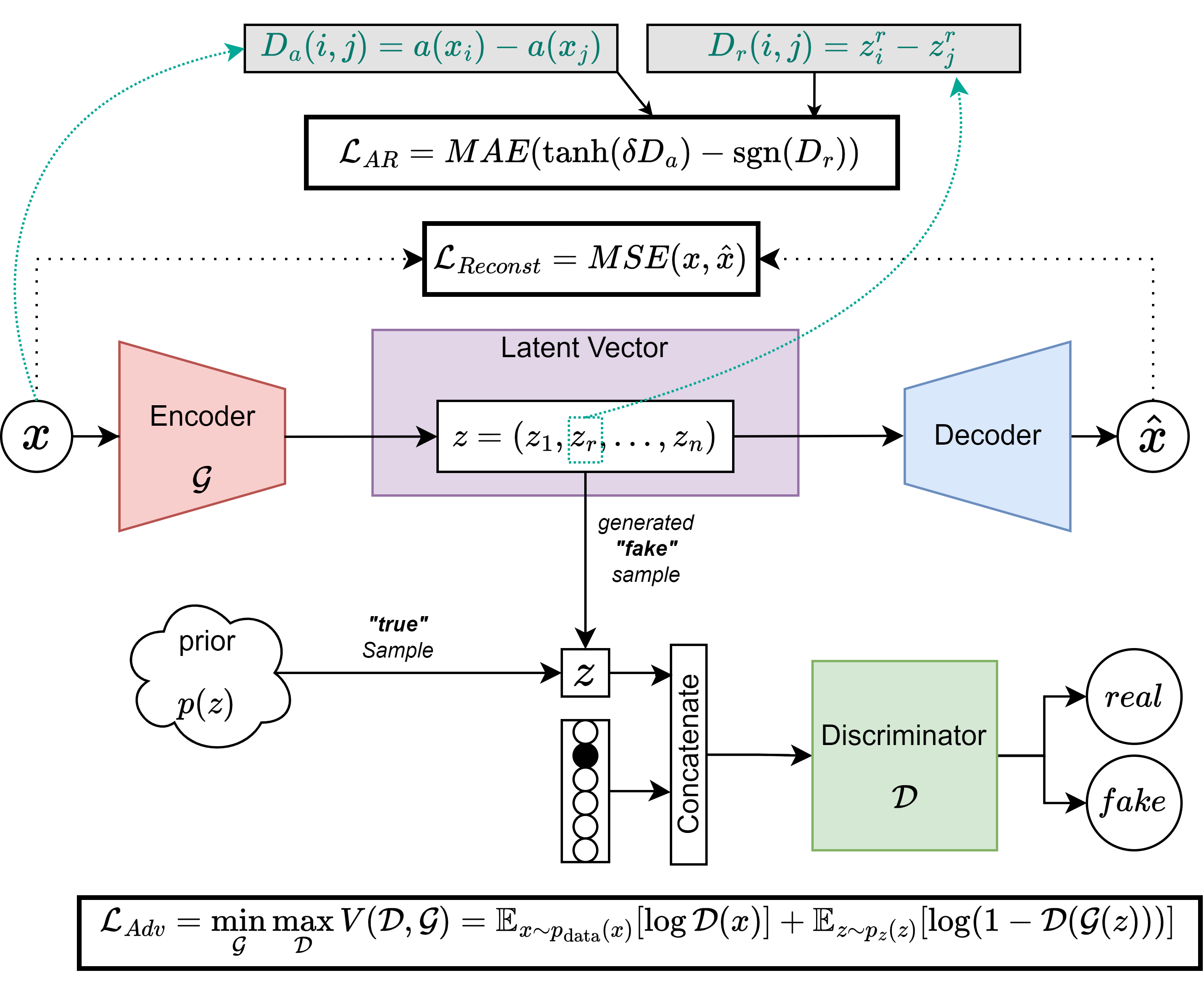
Based on the Adversarial AutoEncoders paper, the model consists of an encoder, a decoder, and a discriminator. The encoder and decoder are the same as in my VAE architecture, and the discriminator is a simple feedforward neural network that takes the latent space vector as input concatenated with a one-hot encoded vector expressing a class variable related to the input sample (bundle of the streamline, neurodegeneration status, etc.) and outputs a single scalar, which is the probability of the input being real or generated. The discriminator is trained to maximize the probability of the real samples and minimize the probability of the generated samples, while the encoder and decoder are trained to minimize the probability of the discriminator being able to distinguish between real and generated samples. Natively, this architecture supports conditioning the generative process on categorical variables, so it is appropriate for our use case.
The attribute-based regularization (AR) is a term added to the loss function of the encoder, with which we try to tie a continuous attribute of choice found in the data space to a specific dimension of the latent space. To do this, we compute an attribute-distance matrix in the data space (\(D_a\)), and we compute a distance matrix from the chosen dimension of the latent space (\(D_r\)). By minimizing the mean absolute error (MAE) between the two matrices, we force the latent space to be organized in such a way that the chosen dimension is related to the chosen attribute. This way, we can generate samples conditioned on the attribute of choice, e.g.: we can generate a streamline with a specific attribute (length).
After training for 64 epochs to see the progress and tendency of the model, we observed that the best reconstruction loss was very high, whereas the adversarial loss components were relatively low in comparison. I suspected that something was off with the generated samples, so I went on to check the training data reconstruction. To no surprise, the model generated the exact same sample every time, suggesting that the model had fallen into mode collapse, a typical problem with adversarial training.
Objectives in Progress#
Solving the mode collapse issue in the AAE model using two strategies:
Implementing a more complex discriminator architecture, with more layers and units, to increase the capacity of the model to distinguish between real and generated samples.
Implementing a Wasserstein loss function, which is known to be more stable than the original GAN loss function, and to prevent mode collapse.
Validating the AAE with the FiberCup data.
Implementing and integrating the attribute-based regularization component inside the working AAE architecture.
Open Source Tasks#
Apart from my project, I got to contribute to the DIPY project in other ways too:
I opened a PR that got merged into the main DIPY repository, which was a nomenclature issue with spherical harmonics. It took some time to agree on how to solve it, but it was very nice to see that the community was open to discussing the issue and to find a solution that was good for everyone. This was the contribution that gave me access to GSoC with DIPY, and it was a very nice start to the journey. Link to the PR: dipy/dipy#3086
I reviewed the code of my fellow GSoC students Kaustav, Wachiou and Robin. It felt very good to understand their projects and to be able to help them with their work, which is completely different from my project. I also reviewed their blogs and participated in the reviews I got from them. It was very pleasant to see how engaging the community is, and how everyone is willing to help each other.
Lastly, I opened an issue in the dipy.org repository that got solved thanks to a contribution from my mentor Serge.
Future Works#
I plan to continue with this project until I arrive to a satisfactory solution to generate synthetic human tractograms with tuneable age and neurodegeneration status properties. This project has not only been a great learning experience, but it has also been a great challenge and a great addition to my PhD research, so I will for sure continue until I succeed.
To complete the work, I will need to:
Complete the objectives in progress.
Train and validate the models with human tractograms.
Integrate the models into DIPY.
Pull Requests#
Because the work is still in progress, no integration of the final version was done yet. However, a draft Pull Request was created to show the progress of the work in the main DIPY repository. For now, it contains the first validated AE, together with tests for the model class. LINK TO THE PR
Conclusions#
I am super grateful for the opportunity to participate in the Google Summer of Code program with DIPY. This journey has been amazing as learning and research experience. I am proud of the progress I have made and what I have achieved. Nevertheless, this is just the beginning of my journey with this project.
I would like to thank again my mentors, Jon Haitz, Jong Sung and Serge, their time, patience, attention, support, and expertise throughout the program. They have been a key part of my success. On the other hand, I would like to thank my fellow GSoC students, Kaustav, Wachiou, and Robin, for their support and collaboration. It has been a pleasure to work with them and to learn from them.
Weekly Blogging#
My blog posts can be found at DIPY website and Python GSoC Mastodon server.
Timeline#
Date |
Title |
Link |
|---|---|---|
27-05-2024 |
Community Bonding Period Summary and first impressions |
|
31-05-2024 |
Building the AutoEncoder, writing the training loop |
|
07-06-2024 |
Refactoring the AutoEncoder, preliminary results |
|
14-06-2024 |
Replicating training parameters, approaching replication |
|
21-06-2024 |
Weight transfer experiments, hardships, and results! |
|
28-06-2024 |
Vacation, starting with the conditional AutoEncoder |
|
06-07-2024 |
Stuck with the Variational AutoEncoder, problems with Keras |
|
12-07-2024 |
Starting to see the light at the end of the VAE |
|
19-07-2024 |
Further advances with the VAE model |
|
26-07-2024 |
The Conditional VAE implementation |
|
02-08-2024 |
Validating the conditional VAE results |
|
09-08-2024 |
The Adversarial AutoEncoder |
|
16-08-2024 |
Last weeks of the coding phase and admin stuff |