Start wrapping up - Test singularities of kurtosis statistics#
As we are reaching the end of the GSoC coding period, I am starting to wrap up the code that I developed this summer.
When reviewing the code implementing the kurtosis standard statistics, I detected some problems on the performance of the analytical solution of the mean kurtosis function.
In this post, I am reporting how I overcame these issues! This post is extremely relevant for those interested in knowing the full details of the implementation of kurtosis standard measures.
Problematic performance near to function singularities#
As I mentioned in previous posts, the function to compute the mean kurtosis was implemented according to an analytical solution proposed by Tabesh et al., 2011. The mathematical formulas of this analytical solution have some singularities, particularly for cases where the diffusion tensor has equal eigenvalues.
To illustrate these singularities, I am plotting below the diffusion and kurtosis tensors of crossing fiber simulations with different intersection angles. Simulations were performed based on the modules implemented during the GSoC coding period.
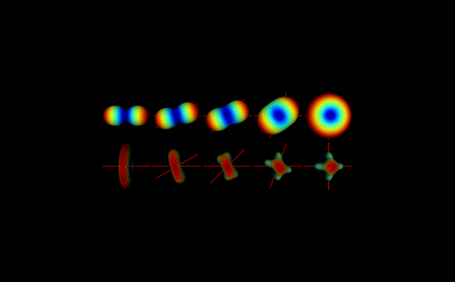
Figure 1 - Diffusion tensor (upper panels) and kurtosis tensors (lower panels) for crossing fibers intersecting at different angles (the ground truth fiber directions are shown in red).#
The values of the eigenvalues of the diffusion tensor as a function of the intersection angle are shown below.
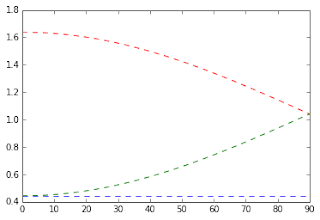
Figure 2 - Diffusion eigenvalues as function of crossing fibers intersection angle. First eigenvalue is plotted in red while the second and third are plotted in green and blue.#
From the figure above, we can detect two problematic cases for the MK analytical solution:
When intersection angle is zero (i.e. when the two fibers are aligned), the second diffusion eigenvalue is equal to the third eigenvalue.
When the intersection angle is 90 degrees, the first diffusion eigenvalue is equal to the second eigenvalue.
Based on the work done by Tabesh et al., 2011, these MK estimation singularities can be mathematically resolved by detecting the problematic cases and using specific formulas for each detected situation. In the previous version of my codes, I was detecting the cases where two or three eigenvalues were equal by analyzing if their differences were three orders of magnitude larger than system’s epsilon. For example, to automatically check if the first eigenvalue equals the second eigenvalue, the following lines of code were used:
import numpy as np
er = np.finfo(L1.ravel()[0]).eps * 1e3
cond1 = (abs(L1 - L2) < er)
Although my testing modules were showing that this procedure was successfully solving the singularities for eigenvalue differences three orders of magnitude smaller than the system’s epsilon, when plotting MK as a function of the intersection angle, some unexpected underestimates were present in the regions near the singularities (see the figures below).
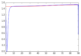
Figure 3 - MK values as function of the crossing angle. The blue line shows the MK values estimated from the analytical solution while the red line shows the MK values estimated from a numerical method described in previous posts.#
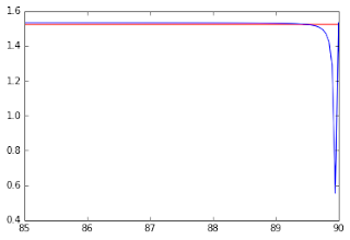
Figure 4 - MK values as function of the crossing angle (range between 85 and 90 degrees). The blue line shows the MK values estimated from the analytical solution while the red line shows the MK values estimated from a numerical method described in previous posts. This figure was produced for a better visualization of the underestimations still present near to the crossing angle of 90 degrees.#
After some analysis, I noticed that MK underestimations were still present if eigenvalues were not 2% different from each other. Given this, I was able to solve this underestimation by adjusting the criteria of eigenvalue comparison. As an example, to compare the first eigenvalue with the second, the following lines of code are now used:
er = 2.5e-2  # difference (in %) between two eigenvalues to be considered as different
cond1 = (abs((L1 - L2) / L1) > er)
Below, I am showing the new MK estimates as a function of the crossing angle, where all underestimations seem to be corrected. Moreover, discontinuities on the limits between the problematic and the non-problematic eigenvalue regime are relatively small. The most significant differences are now between different MK estimation methods (for details on the difference between these methods revisit post #9).
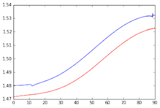
Figure 5 - Corrected MK values as function of the crossing angle. The blue line shows the MK values estimated from the analytical solution while the red line shows the MK values estimated from the numerical method described in previous posts.#